
Automatic Mixed Precision Training
In general, the datatype of training deep learning models is single-precision floating-point format(also called FP32). In 2018, Baidu and NVIDIA jointly published the paper: MIXED PRECISION TRAINING, which proposed mixed precision training. During the process of training, some operators use FP32 and other operators use half precision(also called FP16) in the same time. Its purpose is to speed up training, while compared with the FP32 training model, the same accuracy is maintained. This tutorial will introduce how to use automatic mixed precision training with PaddlePaddle.
1. Half Precision (FP16)
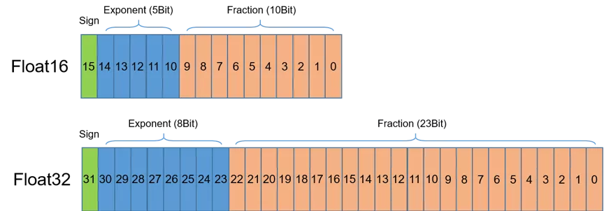
First introduce FP16. As shown in Figure 1, FP16 occupies 16 bits (two bytes in modern computers) of computer memory. In the IEEE 754-2008 standard, it is also named binary16. Compared with FP32 and double precision (also called FP64) commonly used, FP16 is more suitable for the usage in scenarios with low precision requirements.
2. FP16 Computing Power of NVIDIA GPU
When the same hyperparameters are used, mixed precision training using FP16 and FP32 can achieve the same accuracy as that of pure single precision used, and can accelerate the training speed. It mainly attributes to the features that NVIDIA Volta and NVIDIA Turing use FP16 to calculate:
FP16 can reduce memory bandwidth and storage requirements by half, which allows researchers to use more complex models and larger batch sizes under the same hardware conditions.
FP16 can make full use of Tensor Cores technology provided by NVIDIA Volta and NVIDIA Turing. On the same GPU hardware, the computing throughput of Tensor Cores’ FP16 is 8 times bigger than that of FP32.
3. Automatic Mixed Precision Training with PaddlePaddle
Using PaddlePaddle’s API paddle.amp.auto_cast and paddle.amp.GradScaler can realize automatic mixed precision training (AMP), which can automatically choose FP16 or FP32 for different operators’ calculation. After the AMP mode is turned on, the operator list calculated by FP16 and FP32 can be found in this document. This is a specific example to understand how to use PaddlePaddle to achieve mixed precision training.
3.1 Auxiliary Function
First define the auxiliary function to calculate the training time.
import time

# start time
start_time = None

def start_timer():
    # get start time
    global start_time
    start_time = time.time()

def end_timer_and_print(msg):
    # print message and total training time
    end_time = time.time()
    print("\n" + msg)
    print("total time = {:.3f} sec".format(end_time - start_time))
3.2 A Simple Network
Define a simple network to compare the training speed of common methods and mixed precision. The network is composed of three layers of Linear. The first two layers of Linear are followed by the ReLU activation function.
import paddle
import paddle.nn as nn

class SimpleNet(nn.Layer):

    def __init__(self, input_size, output_size):

        super(SimpleNet, self).__init__()
        self.linear1 = nn.Linear(input_size, output_size)
        self.relu1 = nn.ReLU()
        self.linear2 = nn.Linear(input_size, output_size)
        self.relu2 = nn.ReLU()
        self.linear3 = nn.Linear(input_size, output_size)

    def forward(self, x):

        x = self.linear1(x)
        x = self.relu1(x)
        x = self.linear2(x)
        x = self.relu2(x)
        x = self.linear3(x)

        return x
Set the parameters of training. In order to effectively show the improvement of training speed by mixed precision training, please set the larger values of input_size and output_size. And in order to use the Tensor Core provided by GPU, batch_size needs to be set as a multiple of 8.
epochs = 5
input_size = 4096   # set to a larger value
output_size = 4096  # set to a larger value
batch_size = 512    # batch_size is a multiple of 8
nums_batch = 50

train_data = [paddle.randn((batch_size, input_size)) for _ in range(nums_batch)]
labels = [paddle.randn((batch_size, output_size)) for _ in range(nums_batch)]

mse = paddle.nn.MSELoss()
3.3 Training with Default Method
model = SimpleNet(input_size, output_size)  # define model

optimizer = paddle.optimizer.SGD(learning_rate=0.0001, parameters=model.parameters())  # define optimizer

start_timer() # get the start time of training

for epoch in range(epochs):
    datas = zip(train_data, labels)
    for i, (data, label) in enumerate(datas):

        output = model(data)
        loss = mse(output, label)

        # backpropagation
        loss.backward()

        # update parameters
        optimizer.step()
        optimizer.clear_grad()

print(loss)
end_timer_and_print("Default time:") # print massage and total time
Tensor(shape=[1], dtype=float32, place=CUDAPlace(0), stop_gradient=False,
       [1.24072289])

Default time:
total time = 2.935 sec
3.4 Training with AMP
Using automatic mixed precision training with PaddlePaddle requires four steps:
Step1: Define
GradScaler, which is used to scale thelossto avoid underflowStep2: Use
decorate, to do nothing in level=’O1’ mode without using this api, and in level=’O2’ mode to convert network parameters from FP32 to FP16Step3: Use
auto_castto create an AMP context, in which the input datatype(FP16 or FP32) of each oprator will be automatically determinedStep4: Use
GradScalerdefined in Step1 to complete the scaling ofloss, and use the scaledlossfor backpropagation to complete the training
In level=’O1‘ mode:
model = SimpleNet(input_size, output_size)  # define model

optimizer = paddle.optimizer.SGD(learning_rate=0.0001, parameters=model.parameters())  # define optimizer

# Step1:define GradScaler
scaler = paddle.amp.GradScaler(init_loss_scaling=1024)

start_timer() # get start time

for epoch in range(epochs):
    datas = zip(train_data, labels)
    for i, (data, label) in enumerate(datas):

        # Step2:create AMP context environment
        with paddle.amp.auto_cast():
            output = model(data)
            loss = mse(output, label)

        # Step3:use GradScaler complete the loss scaling
        scaled = scaler.scale(loss)
        scaled.backward()

        # update parameters
        scaler.minimize(optimizer, scaled)
        optimizer.clear_grad()

print(loss)
end_timer_and_print("AMP time in O1 mode:")
Tensor(shape=[1], dtype=float32, place=CUDAPlace(0), stop_gradient=False,
       [1.24848151])

AMP time in O1 mode:
total time = 1.299 sec
In level=’O2’ mode:
model = SimpleNet(input_size, output_size)  # define model

optimizer = paddle.optimizer.SGD(learning_rate=0.0001, parameters=model.parameters())  # define optimizer

# Step1:define GradScaler
scaler = paddle.amp.GradScaler(init_loss_scaling=1024)

# Step2:in level='O2' mode, convert network parameters from FP32 to FP16
model, optimizer = paddle.amp.decorate(models=model, optimizers=optimizer, level='O2', master_weight=None, save_dtype=None)

start_timer() # get start time

for epoch in range(epochs):
    datas = zip(train_data, labels)
    for i, (data, label) in enumerate(datas):

        # Step3:create AMP context environment
        with paddle.amp.auto_cast(enable=True, custom_white_list=None, custom_black_list=None, level='O2'):
            output = model(data)
            loss = mse(output, label)

        # Step4:use GradScaler complete the loss scaling
        scaled = scaler.scale(loss)
        scaled.backward()

        # update parameters
        scaler.minimize(optimizer, scaled)
        optimizer.clear_grad()

print(loss)
end_timer_and_print("AMP time in O2 mode:")
in ParamBase copy_to func
in ParamBase copy_to func
in ParamBase copy_to func
in ParamBase copy_to func
in ParamBase copy_to func
in ParamBase copy_to func
Tensor(shape=[1], dtype=float32, place=CUDAPlace(0), stop_gradient=False,
       [1.25075114])

AMP time in O2 mode:
total time = 0.888 sec
4. Advanced Usage
4.1 Gradient Accumulation
Gradient accumulation means running a configured number of steps without updating the model variables. Until certain steps, use the accumulated gradients to update the variables.
In automatic mixed precision training, gradient accumulation is also supported, and the usage is as follows:
model = SimpleNet(input_size, output_size)  # define model

optimizer = paddle.optimizer.SGD(learning_rate=0.0001, parameters=model.parameters())  # define optimizer

accumulate_batchs_num = 10 # the batch numbers of gradients accumulation

# define GradScaler
scaler = paddle.amp.GradScaler(init_loss_scaling=1024)

start_timer() # get start time

for epoch in range(epochs):
    datas = zip(train_data, labels)
    for i, (data, label) in enumerate(datas):

        # create AMP context environment
        with paddle.amp.auto_cast():
            output = model(data)
            loss = mse(output, label)

        # use GradScaler complete the loss scaling
        scaled = scaler.scale(loss)
        scaled.backward()

        #  when the accumulated batch is accumulate_batchs_num, update the model parameters
        if (i + 1) % accumulate_batchs_num == 0:

            # update parameters
            scaler.minimize(optimizer, scaled)
            optimizer.clear_grad()

print(loss)
end_timer_and_print("AMP time:")
Tensor(shape=[1], dtype=float32, place=CUDAPlace(0), stop_gradient=False,
       [1.25853443])

AMP time:
total time = 1.034 sec
5. Conclusion
As can be seen from the above example, using the automatic mixed precision training, in O1 mode the total time is about 1.299s, in O2 mode the total time is about 0.888s, while the ordinary training method takes 2.935s, and the training speed is increased by about 2.4 times in O1 mode and 2.4 times in O2 mode. For more examples of using mixed precision training, please refer to paddlepaddle’s models: paddlepaddle/models.